第八章拉普拉斯变换

第七章：拉普拉斯变换（讲义）

重点：Laplace 变换的性质与应用、逆变换的留数计算法

难点：周期函数和 $\delta$ 函数的变换、留数法求逆变换

7.0 动机：从 Fourier 到 Laplace（单边变换）¶

Fourier 变换在理论与工程中非常重要，但通常要求 $f(t)$ 在 $(-\infty,+\infty)$ 上绝对可积。很多常见函数（常数、多项式、正弦余弦等）不满足该条件；并且许多工程信号只关心 $t\ge 0$ 的响应（初值问题、因果系统），对 $t<0$ 的取值要么没有定义、要么没有意义。

Fourier 的限制与 Laplace 的引入（1）

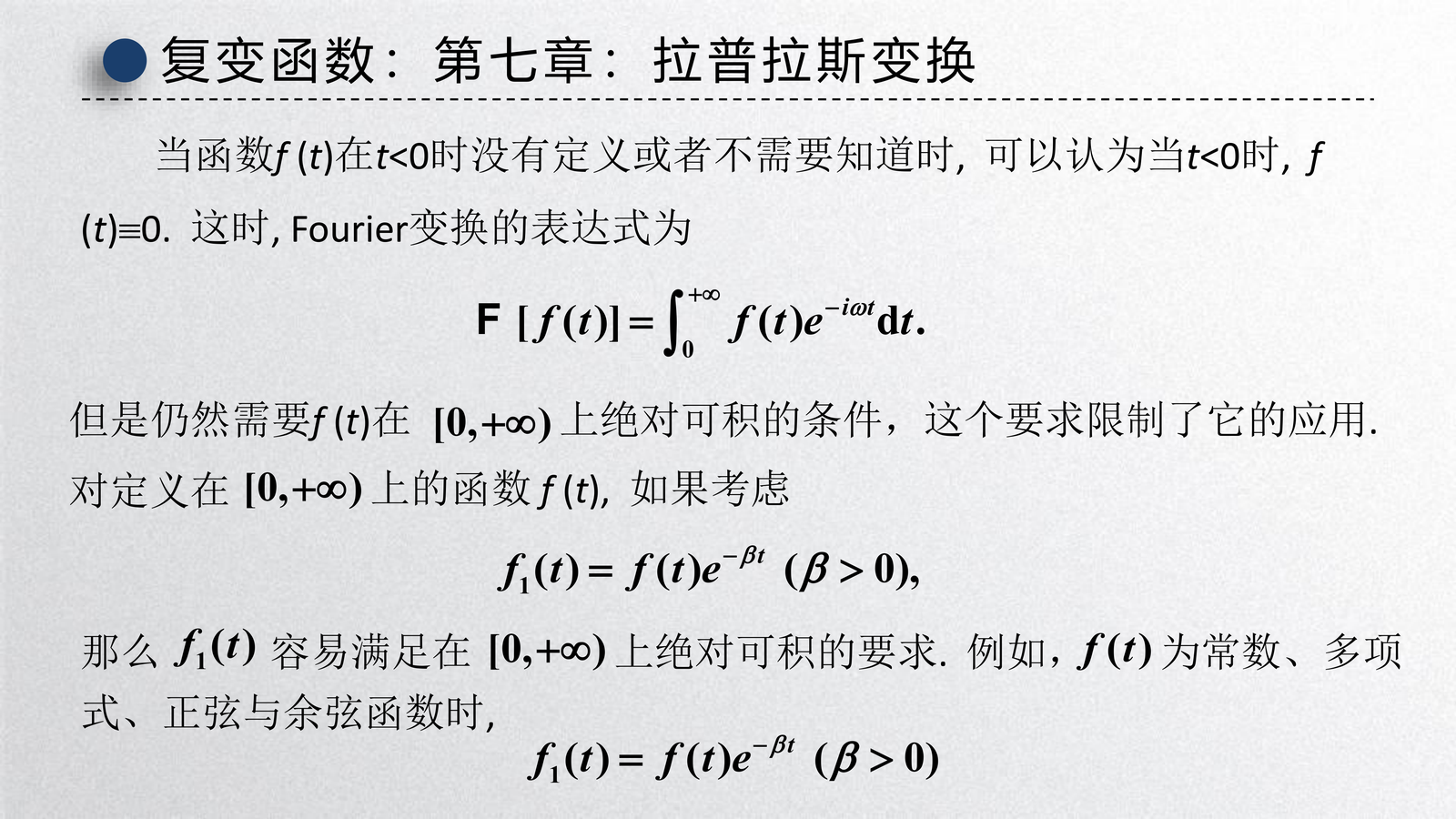
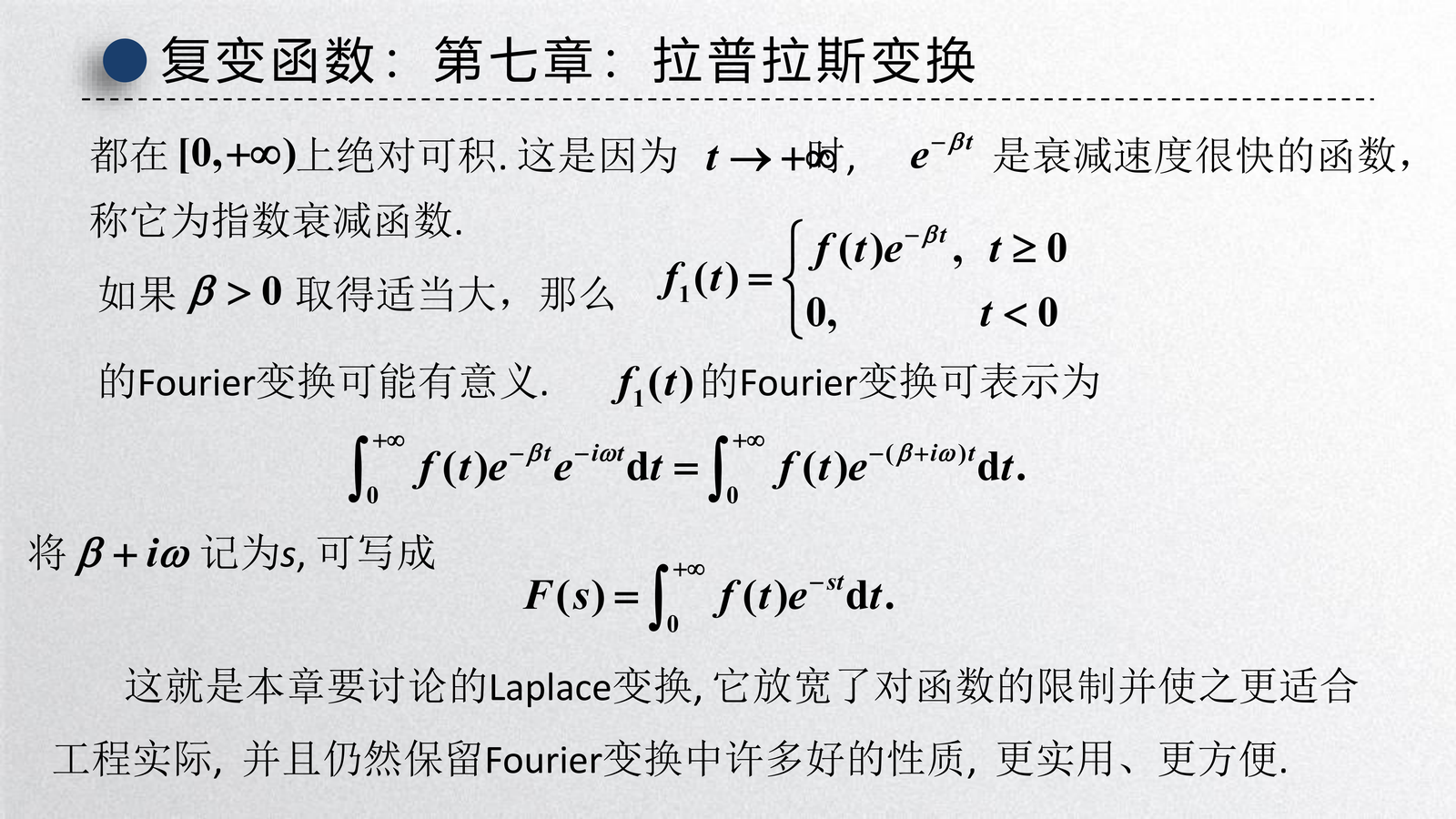
讲义的核心思路是：对 $t\ge 0$ 的函数 $f(t)$，引入一个指数衰减因子 $e^{-\beta t}$（$\beta>0$）把增长“压住”，使其更容易绝对可积。于是类似 Fourier 变换的积分变为

\[ \int_0^{+\infty} f(t)e^{-\beta t}e^{-i\omega t}\,\mathrm{d}t = \int_0^{+\infty} f(t)e^{-(\beta+i\omega)t}\,\mathrm{d}t. \]

记 $s=\beta+i\omega$，就得到 Laplace 变换的标准形式：

$从指数衰减到 $s=\beta+i\omega$（2）$

这解释了两个关键点：

Laplace 变换本质上是在 Fourier 框架里把频率轴“推”到复平面 $s=\sigma+i\omega$ 上，从而显著放宽可积性要求。
工程里常用的是 单边（unilateral）Laplace：把 $t<0$ 视为 $0$，尤其适合初值问题与因果系统。

7.1 Laplace 变换的概念¶

定义与存在定理¶

定义 1（Laplace 变换）

设函数 $f(t)$ 在 $t \geq 0$ 上有定义，且积分

\[ \mathcal{L}[f(t)] = F(s) = \int_0^{+\infty} f(t)e^{-st} \, \mathrm{d}t \]

在复参数 $s$ 的某一区域内收敛，则称 $F(s)$ 为 $f(t)$ 的 Laplace 变换（像函数），$f(t)$ 为 $F(s)$ 的 像原函数。

$单边 Laplace 与 $t<0$ 的约定$

单边（unilateral）与双边（bilateral）Laplace

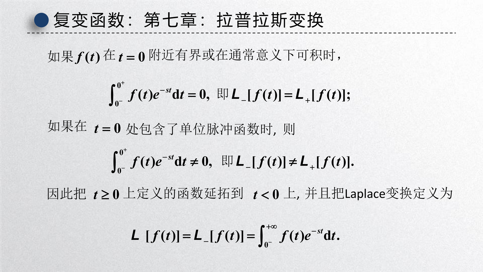
本章默认采用单边 Laplace：只积分 $t\ge 0$ 的部分，因此非常适合处理初值问题。若 $f(t)$ 在 $t=0$ 附近可积且无冲激项，通常可以把 $t<0$ 处延拓为 $0$ 而不影响变换结果；但若 $t=0$ 处含有 $\delta(t)$ 等冲激项，则需要特别注意 $t=0$ 的贡献。

定理 1（Laplace 变换存在定理）

若函数 $f(t)$ 满足：

在 $t \geq 0$ 的任一有限区间上 分段连续
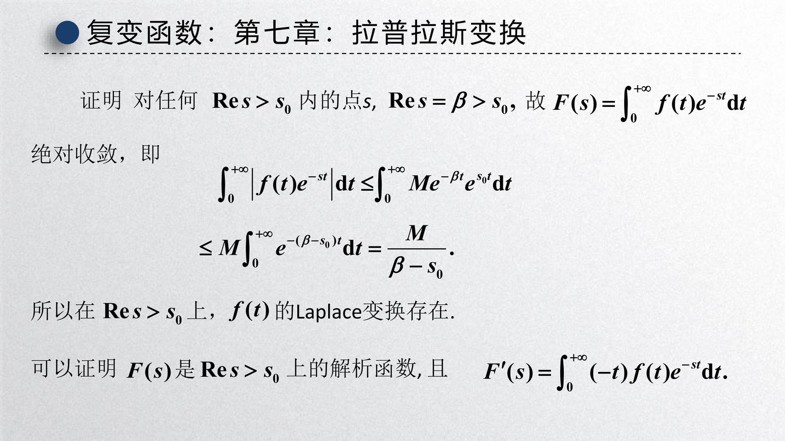
当 $t \to +\infty$ 时，$f(t)$ 的 增长指数 不超过某一指数函数，即存在常数 $M > 0$，$\sigma_0 \geq 0$，使得

\[ |f(t)| \leq Me^{\sigma_0 t}, \quad t \geq 0 \]

则 $f(t)$ 的 Laplace 变换在 半平面 $\text{Re}(s) > \sigma_0$ 上 存在且解析。

其中 $\sigma_0$ 称为 $f(t)$ 的 增长指数。

存在性与解析性（证明思路）

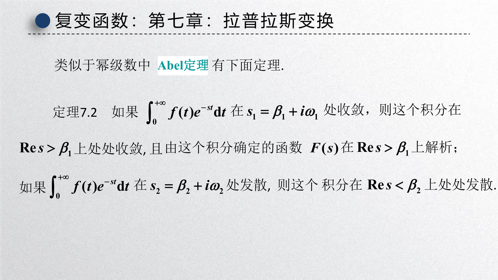
定理 1.1（Abel 型收敛定理与收敛半平面）

若积分 $\int_0^{+\infty} f(t)e^{-st}\,\mathrm{d}t$ 在 $s_1=\beta_1+i\omega_1$ 处收敛，则它在半平面 $\text{Re}(s)>\beta_1$ 上处处收敛，且由该积分确定的像函数 $F(s)$ 在该半平面上解析；若它在 $s_2=\beta_2+i\omega_2$ 处发散，则它在 $\text{Re}(s)<\beta_2$ 上处处发散。

收敛半平面与 Abel 型结论

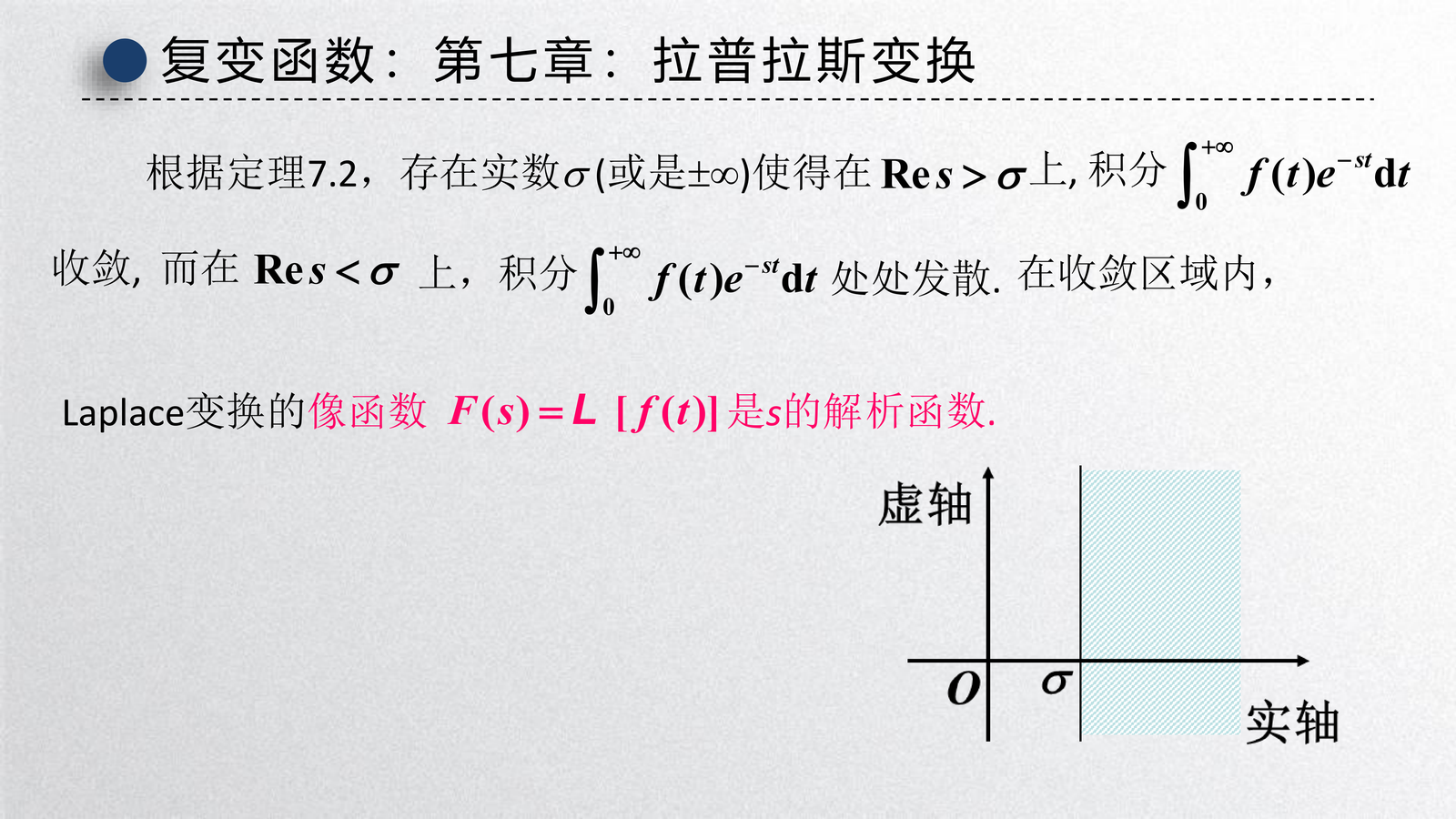
收敛域（ROC）与收敛指数 $\sigma$

由上一结论可知：存在一个实数 $\sigma$（可能为 $\pm\infty$），使得

当 $\text{Re}(s)>\sigma$ 时，$\int_0^{+\infty} f(t)e^{-st}\,\mathrm{d}t$ 收敛
当 $\text{Re}(s)<\sigma$ 时，该积分发散

且在收敛域内像函数 $F(s)=\mathcal{L}[f(t)]$ 是 $s$ 的解析函数。

$收敛指数 $\sigma$ 与 ROC$

基本变换对¶

例 1：单位阶跃函数 $u(t)$

\[ \mathcal{L}[u(t)] = \int_0^{+\infty} e^{-st} \, \mathrm{d}t = \frac{1}{s}, \quad \text{Re}(s) > 0 \]

例 2：指数函数 $e^{at}$

\[ \mathcal{L}[e^{at}] = \int_0^{+\infty} e^{at}e^{-st} \, \mathrm{d}t = \int_0^{+\infty} e^{-(s-a)t} \, \mathrm{d}t = \frac{1}{s-a}, \quad \text{Re}(s) > \text{Re}(a) \]

例 3：正弦函数 $\sin\omega t$ 和余弦函数 $\cos\omega t$

利用 $\sin\omega t = \frac{e^{i\omega t} - e^{-i\omega t}}{2i}$：

\[ \mathcal{L}[\sin\omega t] = \frac{1}{2i}\left(\frac{1}{s-i\omega} - \frac{1}{s+i\omega}\right) = \frac{\omega}{s^2 + \omega^2}, \quad \text{Re}(s) > 0 \]

同理：

\[ \mathcal{L}[\cos\omega t] = \frac{s}{s^2 + \omega^2}, \quad \text{Re}(s) > 0 \]

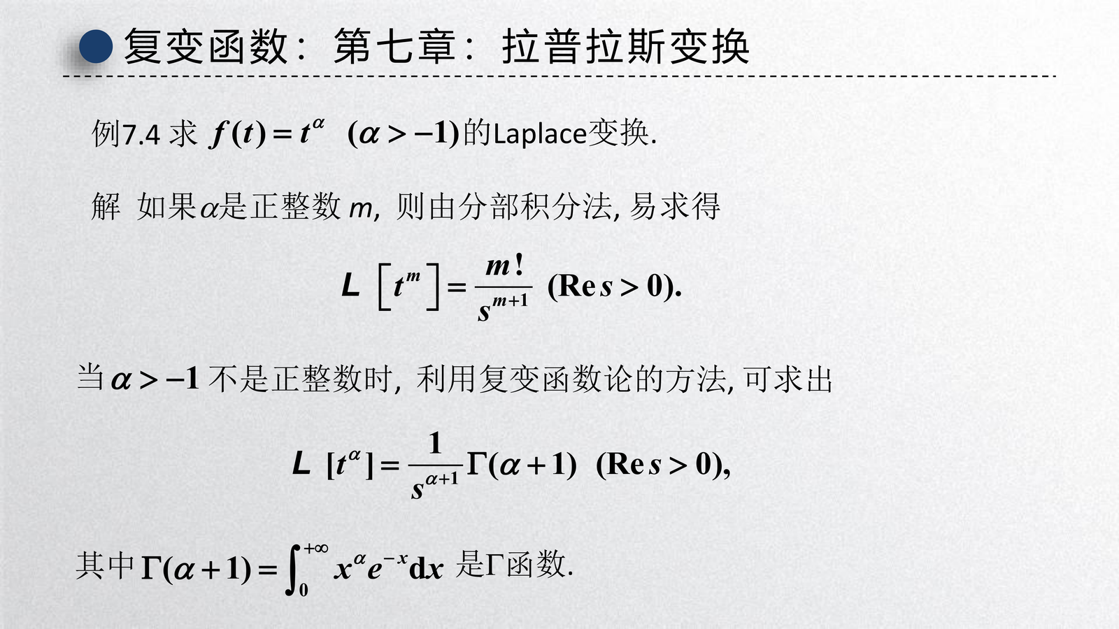
例 4：幂函数 $t^n$（$n$ 为正整数）

利用分部积分：

\[ \mathcal{L}[t^n] = \frac{n!}{s^{n+1}}, \quad \text{Re}(s) > 0 \]

特别地，$\mathcal{L}[1] = \frac{1}{s}$，$\mathcal{L}[t] = \frac{1}{s^2}$。

对于一般幂函数 $t^\alpha$（$\alpha > -1$）：

\[ \mathcal{L}[t^\alpha] = \frac{\Gamma(\alpha+1)}{s^{\alpha+1}} \]

其中 $\Gamma(s)$ 为 Gamma 函数。

幂函数与 Gamma 函数（讲义）

常用 Laplace 变换对表¶

$f(t)$	$F(s) = \mathcal{L}[f(t)]$	收敛域
$1$	$\frac{1}{s}$	$\text{Re}(s) > 0$
$t^n$（$n = 0, 1, 2, \ldots$）	$\frac{n!}{s^{n+1}}$	$\text{Re}(s) > 0$
$e^{at}$	$\frac{1}{s-a}$	$\text{Re}(s) > \text{Re}(a)$
$\sin\omega t$	$\frac{\omega}{s^2 + \omega^2}$	$\text{Re}(s) > 0$
$\cos\omega t$	$\frac{s}{s^2 + \omega^2}$	$\text{Re}(s) > 0$
$\sinh\omega t$	$\frac{\omega}{s^2 - \omega^2}$	$\text{Re}(s) >
$\cosh\omega t$	$\frac{s}{s^2 - \omega^2}$	$\text{Re}(s) >
$t\sin\omega t$	$\frac{2\omega s}{(s^2 + \omega^2)^2}$	$\text{Re}(s) > 0$
$t\cos\omega t$	$\frac{s^2 - \omega^2}{(s^2 + \omega^2)^2}$	$\text{Re}(s) > 0$
$e^{at}\sin\omega t$	$\frac{\omega}{(s-a)^2 + \omega^2}$	$\text{Re}(s) > \text{Re}(a)$
$e^{at}\cos\omega t$	$\frac{s-a}{(s-a)^2 + \omega^2}$	$\text{Re}(s) > \text{Re}(a)$

周期函数和 $\delta$ 函数的 Laplace 变换¶

周期函数的变换¶

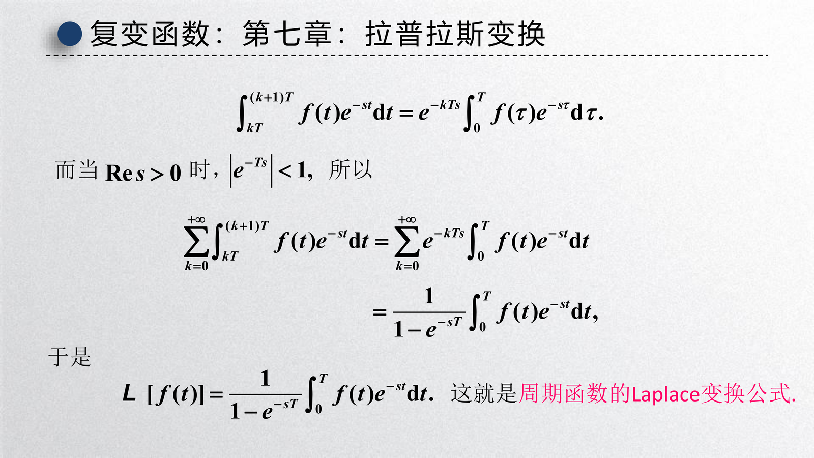
定理 2（周期函数的 Laplace 变换）

设 $f(t)$ 是以 $T$ 为周期的函数，则

\[ \mathcal{L}[f(t)] = \frac{1}{1 - e^{-sT}} \int_0^T f(t)e^{-st} \, \mathrm{d}t \]

周期函数公式推导（讲义）

例 5：全波整流函数 $f(t) = |\sin t|$

周期 $T = \pi$，在 $[0, \pi]$ 上 $f(t) = \sin t$：

\[ \mathcal{L}[|\sin t|] = \frac{1}{1 - e^{-\pi s}} \int_0^\pi \sin t \cdot e^{-st} \, \mathrm{d}t = \frac{1 + e^{-\pi s}}{(1 - e^{-\pi s})(s^2 + 1)} \]

单位脉冲函数 $\delta(t)$¶

定义 2（单位脉冲函数/Dirac delta 函数）

单位脉冲函数 $\delta(t)$ 定义为：

\[ \delta(t) = \begin{cases} 0, & t \neq 0 \\ \infty, & t = 0 \end{cases}, \quad \int_{-\infty}^{+\infty} \delta(t) \, \mathrm{d}t = 1 \]

筛选性质：$\int_{-\infty}^{+\infty} f(t)\delta(t-t_0) \, \mathrm{d}t = f(t_0)$

例 6：$\delta(t)$ 的 Laplace 变换

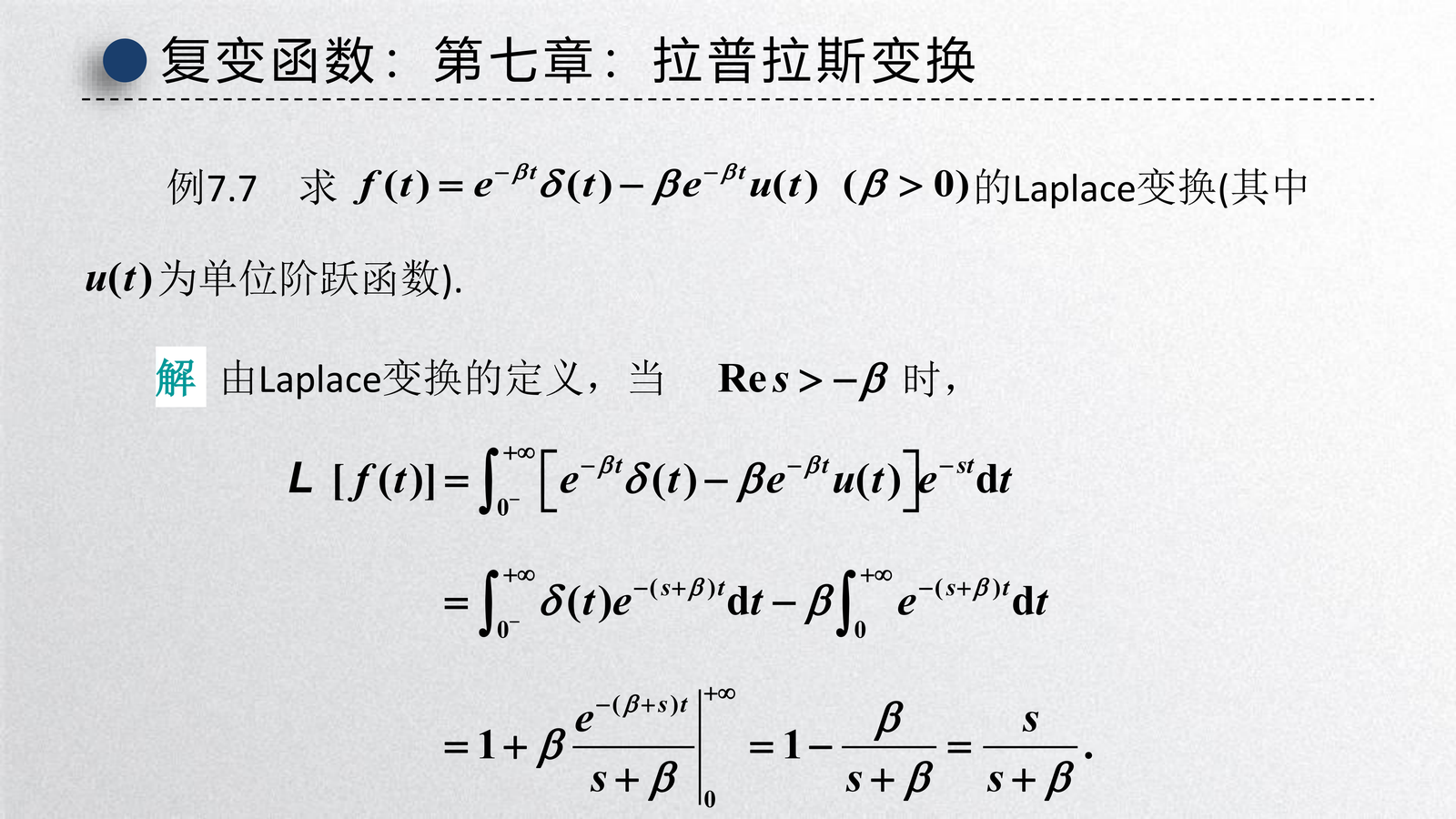
\[ \mathcal{L}[\delta(t)] = \int_0^{+\infty} \delta(t)e^{-st} \, \mathrm{d}t = e^{-s \cdot 0} = 1 \]

例 7：含延迟脉冲函数的变换

\[ \mathcal{L}[\delta(t - t_0)] = e^{-st_0}, \quad t_0 > 0 \]

$含 $\delta(t)$ 的例子（讲义）$

关于 $\delta(t)$ 的几个常用记忆点

记住下面三点：

$\delta(t)$ 是广义函数（分布），它用“筛选性质”刻画：$\int f(t)\delta(t-t_0)\,\mathrm{d}t=f(t_0)$。
与单位阶跃函数的关系：在分布意义下 $u'(t)=\delta(t)$，因此在处理含跳变输入的微分方程时，$\delta$ 往往表示“瞬时冲击”。
单边 Laplace 中，若 $t=0$ 处包含冲激项，需注意 $t=0$ 附近的积分贡献（讲义有专门说明）。

7.2 Laplace 变换的性质¶

十大基本性质¶

1. 线性性质¶

性质 1（线性）： $$ \mathcal{L}[\alpha f_1(t) + \beta f_2(t)] = \alpha F_1(s) + \beta F_2(s) $$

2. 微分性质¶

性质 2（微分）： $$ \mathcal{L}[f'(t)] = sF(s) - f(0) $$

一般地：

\[ \mathcal{L}[f^{(n)}(t)] = s^nF(s) - s^{n-1}f(0) - s^{n-2}f'(0) - \cdots - f^{(n-1)}(0) \]

例 8：用微分性质求 $\mathcal{L}[\cos\omega t]$

因 $(\sin\omega t)' = \omega\cos\omega t$，故

\[ \mathcal{L}[\cos\omega t] = \frac{1}{\omega}\mathcal{L}[(\sin\omega t)'] = \frac{1}{\omega}(s \cdot \frac{\omega}{s^2+\omega^2} - 0) = \frac{s}{s^2+\omega^2} \]

3. 像函数的微分性质¶

性质 3（像函数的微分）： $$ F'(s) = -\mathcal{L}[tf(t)] \quad \text{即} \quad \mathcal{L}[tf(t)] = -F'(s) $$

一般地：$\mathcal{L}[t^nf(t)] = (-1)^n F^{(n)}(s)$。

例 10：求 $\mathcal{L}[t\sin\omega t]$

已知 $\mathcal{L}[\sin\omega t] = \frac{\omega}{s^2+\omega^2}$

\[ \mathcal{L}[t\sin\omega t] = -\frac{\mathrm{d}}{\mathrm{d}s}\left(\frac{\omega}{s^2+\omega^2}\right) = \frac{2\omega s}{(s^2+\omega^2)^2} \]

4. 积分性质¶

性质 4（积分）： $$ \mathcal{L}\left[\int_0^t f(\tau) \, \mathrm{d}\tau\right] = \frac{F(s)}{s} $$

5. 像函数的积分性质¶

性质 5（像函数的积分）：若 $\lim_{t \to 0^+} \frac{f(t)}{t}$ 存在，则

\[ \mathcal{L}\left[\frac{f(t)}{t}\right] = \int_s^{+\infty} F(u) \, \mathrm{d}u \]

例 13：求 $\mathcal{L}\left[\frac{\sin t}{t}\right]$ 及 $\int_0^{+\infty} \frac{\sin t}{t} \, \mathrm{d}t$

\[ \mathcal{L}\left[\frac{\sin t}{t}\right] = \int_s^{+\infty} \frac{1}{u^2+1} \, \mathrm{d}u = \arctan u \bigg|_s^{+\infty} = \frac{\pi}{2} - \arctan s = \arctan\frac{1}{s} \]

令 $s = 0$：

\[ \int_0^{+\infty} \frac{\sin t}{t} \, \mathrm{d}t = \frac{\pi}{2} \]

6. 位移性质¶

性质 6（位移）： $$ \mathcal{L}[e^{at}f(t)] = F(s - a) $$

例 11：求 $\mathcal{L}[e^{at}\sin\omega t]$

\[ \mathcal{L}[e^{at}\sin\omega t] = \frac{\omega}{(s-a)^2 + \omega^2} \]

7. 延迟性质¶

性质 7（延迟）：设 $f(t) = 0$（$t < 0$），则 $\mathcal{L}[f(t - \tau)] = e^{-s\tau}F(s)$（$\tau > 0$）。

8. 相似性质¶

性质 8（相似）： $$ \mathcal{L}[f(at)] = \frac{1}{a}F\left(\frac{s}{a}\right), \quad a > 0 $$

9. 初值和终值定理¶

性质 9（初值和终值定理）：

初值定理：$f(0^+) = \lim_{t \to 0^+} f(t) = \lim_{s \to \infty} sF(s)$
终值定理（若 $\lim_{t \to +\infty} f(t)$ 存在）：$\displaystyle\lim_{t \to +\infty} f(t) = \lim_{s \to 0} sF(s)$

10. 卷积定理¶

定义 3（卷积）：函数 $f_1(t)$ 和 $f_2(t)$ 的卷积定义为

\[ (f_1 * f_2)(t) = \int_0^t f_1(\tau)f_2(t-\tau) \, \mathrm{d}\tau \]

性质 10（卷积定理）：

\[ \mathcal{L}[f_1 * f_2] = F_1(s) \cdot F_2(s) \quad \text{或} \quad \mathcal{L}^{-1}[F_1(s) \cdot F_2(s)] = (f_1 * f_2)(t) \]

卷积定理证明

令 $\tau' = t - \tau$，交换积分次序：

\[ \begin{aligned} \mathcal{L}[f_1 * f_2] &= \int_0^{+\infty} \left[\int_0^t f_1(\tau)f_2(t-\tau) \, \mathrm{d}\tau\right] e^{-st} \, \mathrm{d}t \\ &= \int_0^{+\infty} f_1(\tau) \left[\int_\tau^{+\infty} f_2(t-\tau)e^{-st} \, \mathrm{d}t\right] \, \mathrm{d}\tau \\ &= \int_0^{+\infty} f_1(\tau)e^{-s\tau} \, \mathrm{d}\tau \cdot \int_0^{+\infty} f_2(u)e^{-su} \, \mathrm{d}u \\ &= F_1(s) \cdot F_2(s) \end{aligned} \]

\[\square\]

7.3 Laplace 逆变换¶

反演积分公式¶

反演积分的由来（讲义）

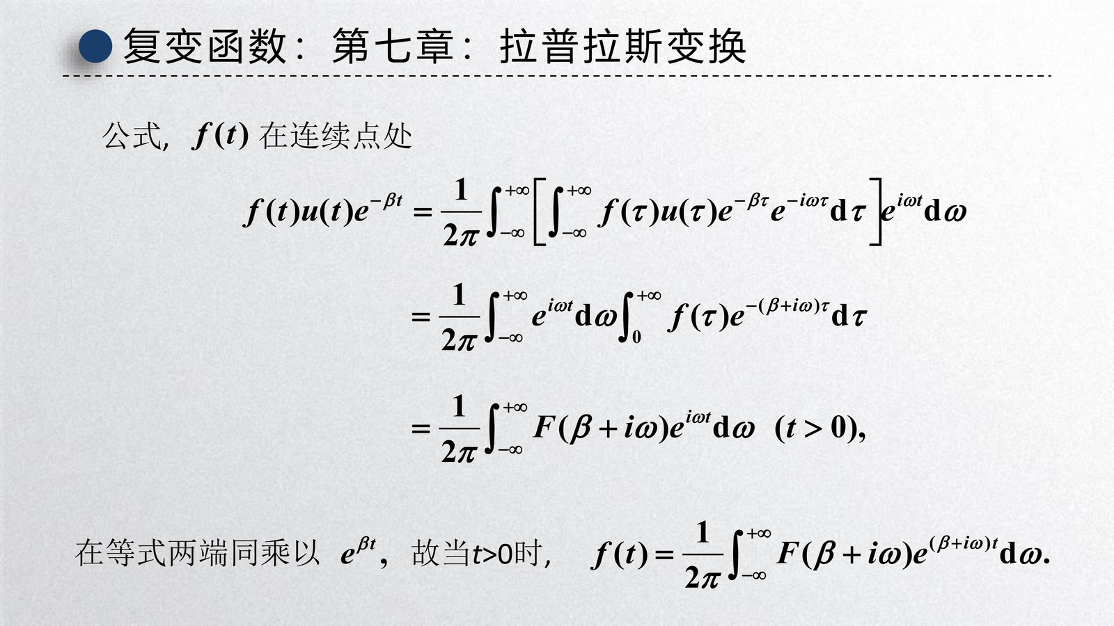
定理 3（反演积分公式）

若 $F(s)$ 是 $f(t)$ 的 Laplace 变换，则

\[ f(t) = \mathcal{L}^{-1}[F(s)] = \frac{1}{2\pi i} \int_{\beta-i\infty}^{\beta+i\infty} F(s)e^{st} \, \mathrm{d}s \]

其中积分路径为复平面上直线 $s = \beta$（$\beta > \sigma_0$，$\sigma_0$ 为 $f(t)$ 的增长指数），方向自下而上。

$\beta$ 取在奇点右侧是什么意思

反演积分路径 $s=\beta$ 通常要求落在 $F(s)$ 的收敛域内（ROC），并且位于 $F(s)$ 的所有孤立奇点右侧。这样在用围道闭合并应用留数时，可以把所有需要贡献的奇点都包进闭合曲线内部。

留数法求逆变换¶

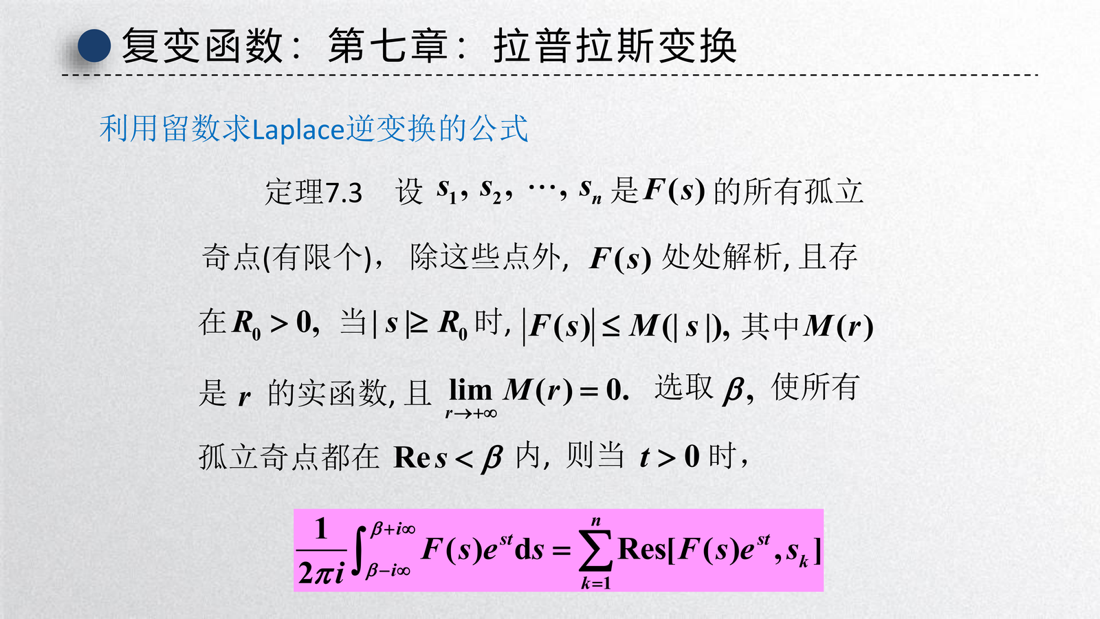
定理 4（留数法）

若 $F(s)$ 在复平面上除有限个孤立奇点 $s_1, s_2, \ldots, s_n$ 外解析，且当 $s \to \infty$ 时 $F(s) \to 0$，则

\[ f(t) = \sum_{k=1}^{n} \text{Res}[F(s)e^{st}, s_k] \]

即 $f(t)$ 等于 $F(s)e^{st}$ 在其所有奇点处留数之和。

利用留数求 Laplace 逆变换（讲义）

例 21：求 $\mathcal{L}^{-1}\left[\frac{1}{s^2+1}\right]$

$F(s)e^{st} = \frac{e^{st}}{s^2+1} = \frac{e^{st}}{(s-i)(s+i)}$ 有奇点 $s = \pm i$

在 $s = i$：

\[ \text{Res} = \lim_{s \to i} (s-i) \cdot \frac{e^{st}}{(s-i)(s+i)} = \frac{e^{it}}{2i} \]

在 $s = -i$：

\[ \text{Res} = \lim_{s \to -i} (s+i) \cdot \frac{e^{st}}{(s-i)(s+i)} = \frac{e^{-it}}{-2i} \]

因此

\[ f(t) = \frac{e^{it}}{2i} - \frac{e^{-it}}{2i} = \sin t \]

例 22：求 $\mathcal{L}^{-1}\left[\frac{1}{s(s-1)^2}\right]$

$F(s)e^{st}$ 有奇点 $s = 0$（一级）和 $s = 1$（二级）

在 $s = 0$：

\[ \text{Res} = \lim_{s \to 0} s \cdot \frac{e^{st}}{s(s-1)^2} = 1 \]

在 $s = 1$：

\[ \text{Res} = \lim_{s \to 1} \frac{\mathrm{d}}{\mathrm{d}s}\left[(s-1)^2 \cdot \frac{e^{st}}{s(s-1)^2}\right] = \lim_{s \to 1} \frac{\mathrm{d}}{\mathrm{d}s}\left(\frac{e^{st}}{s}\right) = te^t - e^t \]

因此

\[ f(t) = 1 + e^t(t-1) \]

7.4 Laplace 变换的应用¶

Laplace 变换的应用（讲义）

求解微分方程¶

基本思路： 1. 对方程两边进行 Laplace 变换 2. 得出像函数的代数方程 3. 求出像函数 4. 通过逆变换得出解

例 26：求解二阶常系数线性微分方程初值问题

\[ x'' - 2x' + 2x = 2e^t\cos t, \quad x(0) = x'(0) = 0 \]

解：设 $\mathcal{L}[x(t)] = X(s)$，对方程两边取 Laplace 变换：

\[ s^2X(s) - 2sX(s) + 2X(s) = \frac{2(s-1)}{(s-1)^2+1} \]

（利用 $\mathcal{L}[e^t\cos t] = \frac{s-1}{(s-1)^2+1}$）

解得：

\[ X(s) = \frac{2(s-1)}{[(s-1)^2+1](s^2-2s+2)} = \frac{2(s-1)}{[(s-1)^2+1]^2} \]

逆变换得：

\[ x(t) = te^t\sin t \]

例 27：求解积分方程

\[ y(t) = at + \int_0^t y(\tau)\sin(t-\tau) \, \mathrm{d}\tau \]

解：设 $\mathcal{L}[y(t)] = Y(s)$，方程化为

\[ Y(s) = \frac{a}{s^2} + Y(s) \cdot \frac{1}{s^2+1} \]

（利用卷积定理）

解得：

\[ Y(s) = \frac{a(s^2+1)}{s^4} = \frac{a}{s^2} + \frac{a}{s^4} \]

逆变换得：

\[ y(t) = at + \frac{a}{6}t^3 \]

电路分析¶

RC 电路¶

例 32：RC 串联电路分析

电路方程：$RC\frac{\mathrm{d}u_C}{\mathrm{d}t} + u_C = E$（$u_C(0) = 0$）

取 Laplace 变换：

\[ RCsU_C(s) + U_C(s) = \frac{E}{s} \]

解得：

\[ U_C(s) = \frac{E}{s(RCs+1)} = E\left(\frac{1}{s} - \frac{1}{s+\frac{1}{RC}}\right) \]

逆变换得：

\[ u_C(t) = E(1 - e^{-\frac{t}{RC}}) \]

RLC 电路¶

例 33：RLC 串联电路分析

电路方程：$LC\frac{\mathrm{d}^2u_C}{\mathrm{d}t^2} + RC\frac{\mathrm{d}u_C}{\mathrm{d}t} + u_C = E$

类似地通过 Laplace 变换求解，根据特征根的不同情况（过阻尼、临界阻尼、欠阻尼）得到不同形式的解。

线性定常系统与传递函数¶

定义 4（传递函数）：传递函数 定义为系统输出与输入的 Laplace 变换之比：

\[ H(s) = \frac{Y(s)}{U(s)} \]

其中 $Y(s)$ 为输出的 Laplace 变换，$U(s)$ 为输入的 Laplace 变换。

多输入多输出系统

对于多输入多输出系统，可用传递函数矩阵描述：

\[ \mathbf{Y}(s) = \mathbf{H}(s)\mathbf{U}(s) \]

其中 $\mathbf{H}(s)$ 为传递函数矩阵。

小结¶

核心公式¶

Laplace 变换定义¶

\[ \mathcal{L}[f(t)] = F(s) = \int_0^{+\infty} f(t)e^{-st} \, \mathrm{d}t \]

基本变换对¶

最常用的 5 个基本变换对

先把下面这 5 个“母公式”记牢：

$1 \;\longleftrightarrow\; \dfrac{1}{s}$
$t^n \;\longleftrightarrow\; \dfrac{n!}{s^{n+1}}$
$e^{at} \;\longleftrightarrow\; \dfrac{1}{s-a}$
$\sin\omega t \;\longleftrightarrow\; \dfrac{\omega}{s^2+\omega^2}$
$\cos\omega t \;\longleftrightarrow\; \dfrac{s}{s^2+\omega^2}$

十大性质速查¶

十大性质速查

下面按“名字 + 公式”直接速记：

线性：$\mathcal{L}[\alpha f_1 + \beta f_2] = \alpha F_1 + \beta F_2$
微分：$\mathcal{L}[f'] = sF(s) - f(0)$
像函数微分：$\mathcal{L}[tf(t)] = -F'(s)$
积分：$\mathcal{L}\!\left[\int_0^t f(\tau)\,\mathrm{d}\tau\right] = \dfrac{F(s)}{s}$
像函数积分：$\mathcal{L}\!\left[\dfrac{f(t)}{t}\right] = \int_s^\infty F(u)\,\mathrm{d}u$
位移：$\mathcal{L}[e^{at}f(t)] = F(s-a)$
延迟：$\mathcal{L}[f(t-\tau)] = e^{-s\tau}F(s)$
相似：$\mathcal{L}[f(at)] = \dfrac{1}{a}F\!\left(\dfrac{s}{a}\right)$
初值定理：$f(0^+) = \lim_{s \to \infty} sF(s)$
终值定理：$\lim_{t \to \infty} f(t) = \lim_{s \to 0} sF(s)$
卷积：$\mathcal{L}[f_1 * f_2] = F_1(s)F_2(s)$

逆变换方法¶

逆变换方法速查

看到像函数 $F(s)$ 时，可以按下面的顺序判断：

部分分式分解：适用于 $F(s)$ 为有理函数
留数法：适用于 $F(s)$ 有孤立奇点
查表法：适用于常见标准形式
卷积定理：适用于 $F(s)=F_1(s)F_2(s)$

应用流程¶

实际问题 → 建立微分/积分方程 → Laplace变换 → 代数方程
                                               ↓
实际解 ← 逆变换 ← 像函数解 ← 求解代数方程

记忆口诀

速记如下：

微分性质：$s$ 乘像函数减初值
位移性质：$s$ 替换为 $s-a$
延迟性质：乘以 $e^{-s\tau}$
卷积定理：时域卷积变频域乘积
逆变换留数法：$F(s)e^{st}$ 的留数之和

\(f(t)\)	\(F(s) = \mathcal{L}[f(t)]\)	收敛域
\(1\)	\(\frac{1}{s}\)	\(\text{Re}(s) > 0\)
\(t^n\)（\(n = 0, 1, 2, \ldots\)）	\(\frac{n!}{s^{n+1}}\)	\(\text{Re}(s) > 0\)
\(e^{at}\)	\(\frac{1}{s-a}\)	\(\text{Re}(s) > \text{Re}(a)\)
\(\sin\omega t\)	\(\frac{\omega}{s^2 + \omega^2}\)	\(\text{Re}(s) > 0\)
\(\cos\omega t\)	\(\frac{s}{s^2 + \omega^2}\)	\(\text{Re}(s) > 0\)
\(\sinh\omega t\)	\(\frac{\omega}{s^2 - \omega^2}\)	$\text{Re}(s) >
\(\cosh\omega t\)	\(\frac{s}{s^2 - \omega^2}\)	$\text{Re}(s) >
\(t\sin\omega t\)	\(\frac{2\omega s}{(s^2 + \omega^2)^2}\)	\(\text{Re}(s) > 0\)
\(t\cos\omega t\)	\(\frac{s^2 - \omega^2}{(s^2 + \omega^2)^2}\)	\(\text{Re}(s) > 0\)
\(e^{at}\sin\omega t\)	\(\frac{\omega}{(s-a)^2 + \omega^2}\)	\(\text{Re}(s) > \text{Re}(a)\)
\(e^{at}\cos\omega t\)	\(\frac{s-a}{(s-a)^2 + \omega^2}\)	\(\text{Re}(s) > \text{Re}(a)\)

7.0 动机：从 Fourier 到 Laplace（单边变换）¶

7.1 Laplace 变换的概念¶

定义与存在定理¶

基本变换对¶

常用 Laplace 变换对表¶

周期函数和 \(\delta\) 函数的 Laplace 变换¶

周期函数的变换¶

单位脉冲函数 \(\delta(t)\)¶

7.2 Laplace 变换的性质¶

十大基本性质¶

1. 线性性质¶

2. 微分性质¶

3. 像函数的微分性质¶

4. 积分性质¶

5. 像函数的积分性质¶

6. 位移性质¶

7. 延迟性质¶

8. 相似性质¶

9. 初值和终值定理¶

10. 卷积定理¶

7.3 Laplace 逆变换¶

反演积分公式¶

留数法求逆变换¶

7.4 Laplace 变换的应用¶

求解微分方程¶

电路分析¶

RC 电路¶

RLC 电路¶

线性定常系统与传递函数¶

小结¶

核心公式¶

Laplace 变换定义¶

基本变换对¶

十大性质速查¶

逆变换方法¶

应用流程¶